Energy Efficiency Prediction:
Analyzing Effects of Local Law 97
1. Introduction
Environmental sustainability has arrived at the forefront of policy in New York City over the past decade as water levels and temperatures climb. Responsible for around 36 percent of the world’s energy use, commercial and residential buildings contribute immensely to this struggle. In 2019, Local Law 97, one of New York City’s more ambitious plans against climate change was passed: incentivizing buildings over 25,000 square feet to meet new energy efficiency standards at the cost of higher taxes. Investigating this policy, I will hope to test its true effectiveness three years into its implementation (with a milestone of 40 percent reduction in greenhouse gas emissions by 2030). By employing data on housing characteristics, location, temperature, and energy output, I will generate many different estimators (OLS, Fixed Effects, Ridge Regression, and Neural Networks) for energy use in building complexes preceding Local Law 97. I can then use my model to predict energy consumption after Local Law 97 against realized outputs to reveal the effectiveness of the policy. Inspired by work from Constantine Kontokosta’s A Data-Driven Predictive Model of City-Scale Energy Use in Buildings, I hope to exercise many machine learning methods to explain with greater insight the relationships between housing features and energy output in New York City, particularly if any movement has been spurred by local proactivity in Local Law 97.
Similar to Kontokosta, I selected optimal features of Borough, Occupancy, and Proportions of Residential, Office, Storage, and Factory square footage to the gross square footage of the building. Kontokosta engaged in a more rigorous effort to determine these powerful features through a fitting series of OLS models. Employing his selected features, I eventually differed in choosing a Neural Network model of dense layers to describe the relationship of the features to Site Energy Use Intensity (kBtu/ft2), my target variable. I ultimately took the natural log of the EUI, assuming a normal relationship between my variables for ease of explanation.
1.1 Prompt
Particularly focusing on residential housing in New York City, employing housing characteristics, location, and temperature, we will investigate the different predictors of energy output before the implementation of Local Law 97: ultimately, comparing our predictor to actual outputs in the years following the passing of Local Law 97.
2. Data Sources and Descriptions
I used the Energy and Water Disclosure for Local Law 84 (EWD: coinciding bill to Local Law 97 for disclosure of outputs and housing characteristics for complexes over 25,000 square feet). Note: After discussing the project in greater depth with Giulia, I decided to not merge an alternate PLUTO dataset on housing features, and would instead pursue solely the EWD.
2.1 Energy and Water Disclosure (Local Law 84)
EWD will provide technical insight into the building’s overall carbon expenditure. With over 300 features, spanning over 30,000 observations in a given year, EWD will be the primary dataset of interest. Its specialization in the decomposition of energy use into tangible metrics qualifies the dataset to lead in supporting the prediction model. Features of the proprietary certification of Energy Star (a prominent energy auditing service in the Northeast), Target Rating of Energy Star, Current Direct Greenhouse Gas Emissions, Current Total On-Site Renewable Electric Use, Percent of Electricity from On-Site Renewable, Total Avoided GHG Emissions from Green Power, and so forth all lend themselves to layering and building up a model that can comprehend the nuances of Energy Use Intensity (EUI, and our dependent variable of interest). Energy Use Intensity follows the unit measurement of kBtu/ft2, recognizing the energy efficiency of the building at hand, and how other endogenous variables listed influence this ultimate target. I would like to also note the use of proportional square footage for the intended use (residential, storage, office, etc.) also provided valuable information on how space was oriented and if that had an influence on energy efficiency.
2.2 Data Organization
The dataset would comprise panel data: the pre-LL97 as 2015-2019; the post-LL97 as 2019-2021. The unit of observation is buildings (based on a unique Property ID for 30,000 observations). The EWD contains yearly data on these buildings, and there seemed to be a small, but notable decrease in the years 2020-2021 in EUI - potentially correlated with the legislation of LL97. I would append five years of data to constitute this pre-LL97 period, and two years as post-LL97. If Property ID, Largest Property Use Type - Gross Square Footage, Borough, and Occupancy were missing values, then those buildings would be dropped - I found this data to be critical in maintaining a complete dataset. All Nans and infinite numbers were dropped. Dummy variables would then be created for Boroughs and Proportions (Residential, Office, Storage, Retail, Factory) as Kontokosta also implemented. I used a bin mechanism to describe the relative proportions of these spaces to the gross (0-.25, .25-.50, .50-.75,.75-1.0). The column ‘year’, which was integrated for the panel’s sake, was altered as a linear time trend in relation to the Site EUI. Thus, the pre-LL97 year would take a number between 0-5, and the post-LL97 year would take a number between 6-7.
3. Methodology
3.1 Machine Learning Techniques (Developing a control group)
I attempted estimator techniques of Fixed Effects on my OLS linear regression and found an optimal expression in a non-linear relationship through Neural Networks.
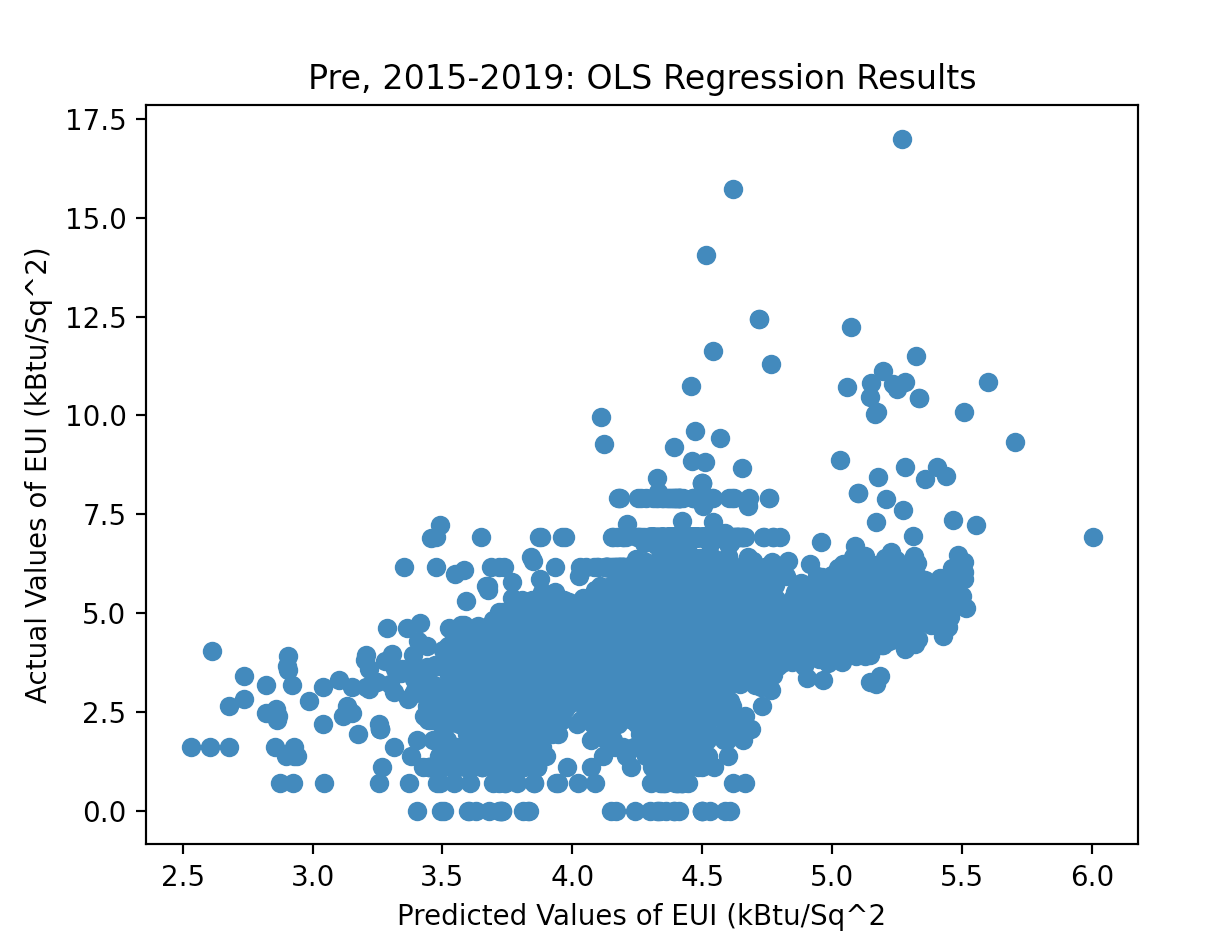
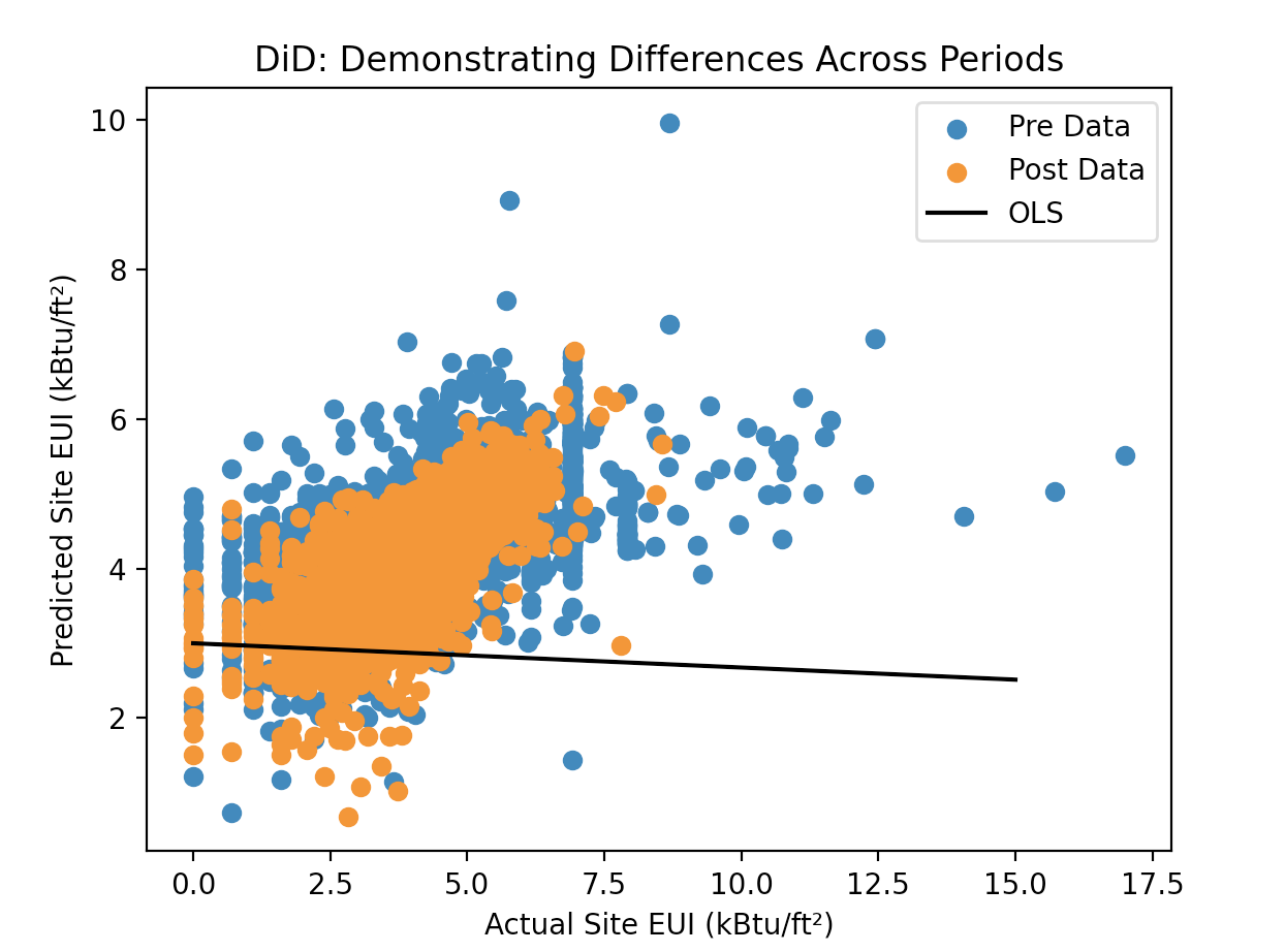
The OLS technique (Figures 3-4 and from non-disclosed tests) demonstrates the underfitted relationship of these features against Site EUI. As demonstrated in Figures (3-4), the OLS overpredicts in the post-period and underpredicts in the pre-period. The R^2 for both of these regressions falls under .23 (pre) and .32 (post), indicating again an underfitting of the data. However, under the respective model summaries, there is evidence of significant p-values across many features. Notably, having no space partitioned for multi-family occupation would have as impactful as a 1-point shift in Site EUI. With that variable thus accounting for the greatest magnitude towards Site EUI it is worth wondering how correlated these features may be. Figure (2), a Collinearity matrix of all the features, expands on this check. There are in fact notably low correlations between many of the features, entertaining the reasonable assumption that OLS does not in fact classify the data particularly well.
As noted in Figure (1), a distribution of the Site EUI Test Data, there is a cluster of more than one-sixth of the dataset aligned to a Site EUI of around 5. Trained on data that would likely point to a Site EUI of 5, with significant shifts on an exponential scale for any movement around this point because of the natural log behavior. Thus, the model predominantly provides a cluster around this range: [4,6]. Outliers in the dataset are noticeable in the pre-period, never predicting over the Site EUI of 6.0. Interestingly, these outliers are condensed and not present in the post-period. These observations were supportive in providing greater texture to the dynamic features that I was employing. Thus, I proposed employing neural networks to explain non-linear relationships between my regressors and EUI.
Initially, I had hoped to optimize my Neural Network with a Ridge Regression (which after discussing with Giulia, I decided to drop for time purposes), but was unable to straddle the Bias-Complexity dilemma. I thus developed a hypothesis through a fully connected Neural Network of five dense layers and a dropout regularizer. I chose epochs of around 50, as I noticed that my validation loss began to increase above that time frame, and did not wish to overfit my training data. The learning rate remained at .001 for similar purposes, and an Adams optimizer was selected. The loss function of Mean Squared Error was selected (achieving .4538 testing loss on the pre-period data; achieving .2045 testing loss on the post-period data). I believe that my hypothesis describes the data relatively well, but struggled with scaling my variables and reading into deeper insights concerning the marginal effects of each feature on the target.
3.2 Average Treatment Effect
Because the nature of this project is based on understanding the greater causation of our policy Local Law 97 in mitigating carbon emissions, an Average Treatment Effect must be undertaken. In applying Hal Varian’s tools for navigating a time series problem, we realize that we must employ an OLS regression model to find the differences (DiD) between the groups. Two years since Local Law 97 was implemented, these years will provide an interaction of time and the actual policy: both describing two differences that could suggest an actual effect of Local Law 97. I ultimately found a DiD of -0.09, which is unfortunately not significant enough to represent movement in the Site EUI.
4. Expected Results / Conclusions
In implementing a Neural Network on the EWD since the implementation of Local Law 97 in 2019, there seems to not be a meaningful difference in EUI across time: indicating that Local Law 97 has not yet impacted Site EUI. I believe that my predictive model suggested a control group post-2019 that ultimately demonstrated marginally small differences in energy consumption and behavior. Although the model arrived at this conclusion, I will note the difficulty in representing the data through my network and found little shifts in the data. This endeavor hoped to investigate the implications of building environment (Borough, Floor Purposing, Occupancy) in explaining a building’s potential affinity to GHG change post-Local Law 97. While not the focus by any means, these extra details may shed light on this ultimate movement toward sustainable infrastructure. Unfortunately, the effect of Local Law 97 may be still nascent, but perhaps the emergence and power of green policy will take up greater force in the coming years.
5. Code Repository
Our codebase is accessible on GitHub at: https://github.com/okanders/energy-efficiency-LL97
6. References:
- Kontokosta, Constantine & Tull, Christopher. (2017). A data-driven predictive model of city-scale energy use in buildings. Applied Energy. 197. 303-317. 10.1016/j.apenergy.2017.04.005.
- Hal R. Varian, 2014. "Big Data: New Tricks for Econometrics," Journal of Economic Perspectives, American Economic Association, vol. [Volume and pages if available]
- PLUTO: BYTES of the BIG APPLE™ - Archive. https://www.nyc.gov/site/planning/data-maps/open-data/bytes-archive.page
- Energy and Water Disclosure - Local Law 84. https://data.cityofnewyork.us/browse?q=Local+Law+84
7. Appendix
Figure (1): Distribution of Site EUI in Test Set
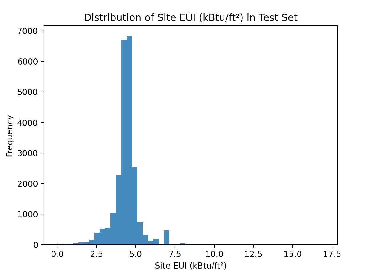
Figure (2): Collinearity Matrix of Predictors and Dummy Variables
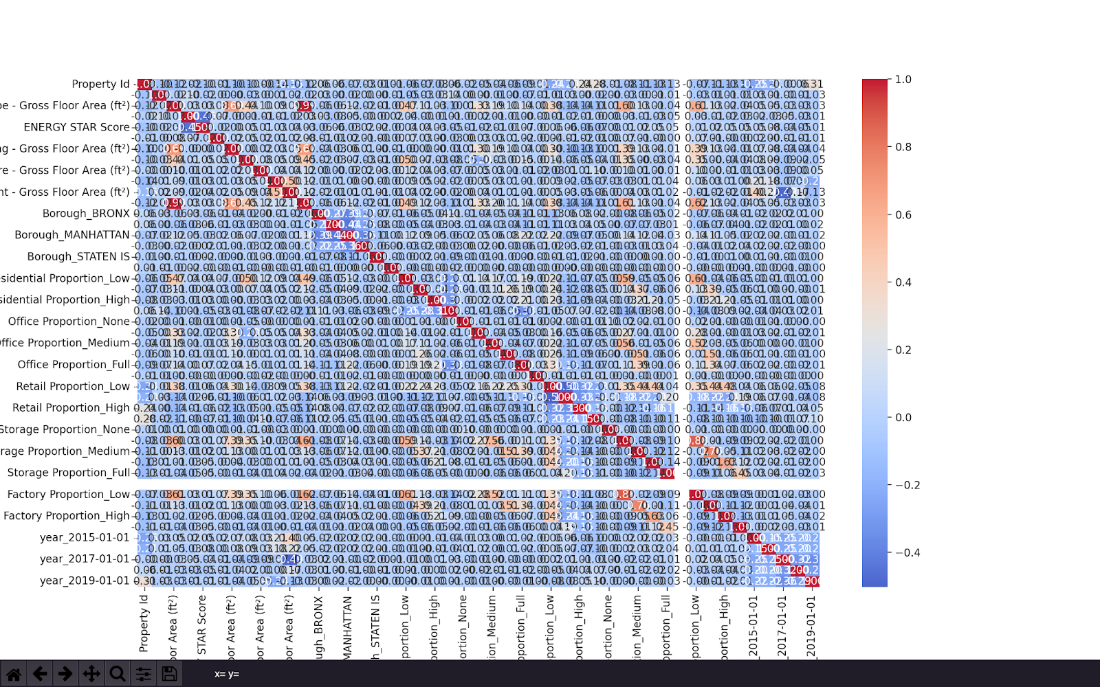
Figure (3): OLS Regression on Post-LL97 Data; 2020-2021
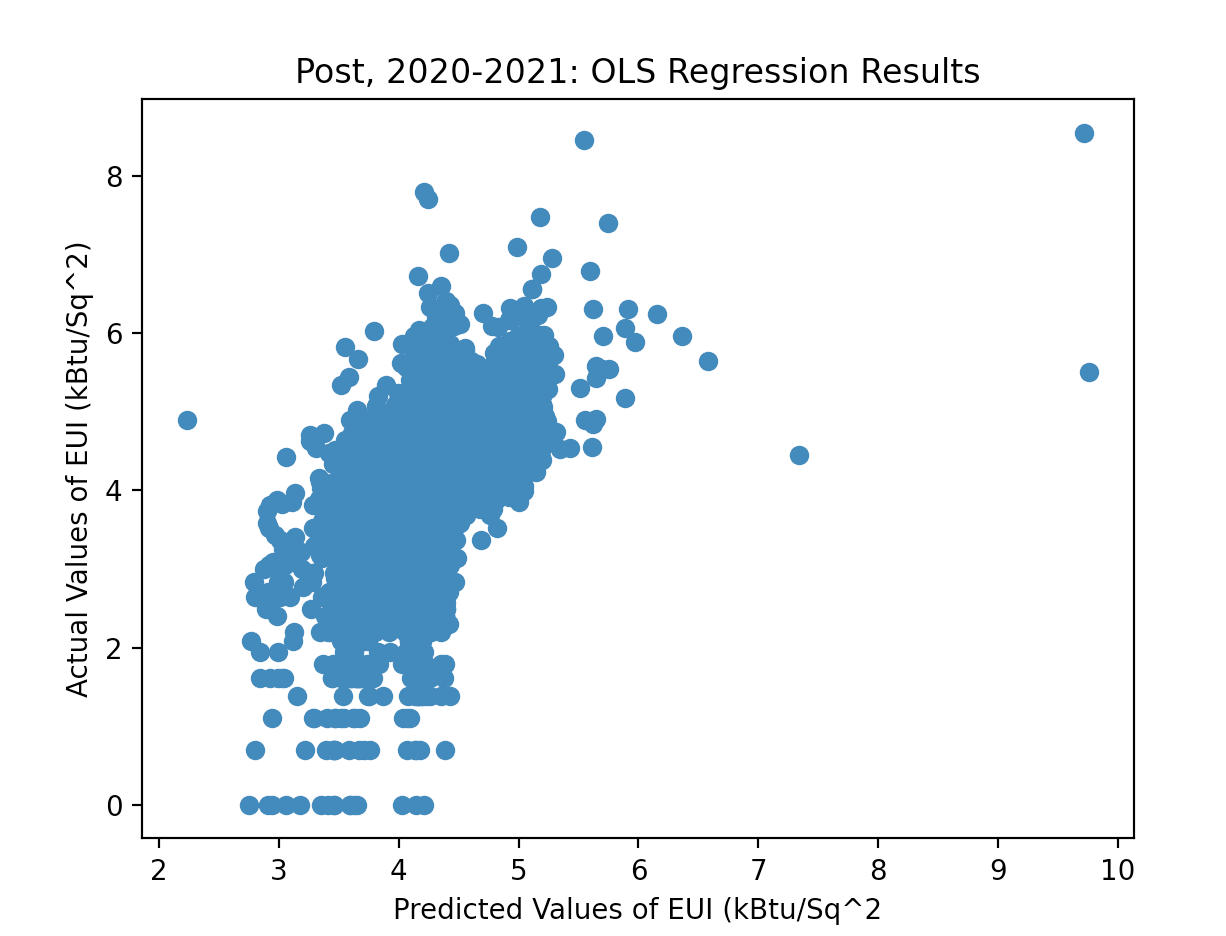
Figure (4): OLS Regression on Pre-LL97 Data; 2020-2021